Extinction Suite Macro (v4.1.5) for ImageJ (2011-2021)
Written by Lukas Payne (LP)
Acknowledgements
- David Coffin for the DCRAW reader plugin, and any
contributors to ImageJ's original batch converter plugin.
- Wolfgang Langbein and Paola Borri for supervision and advice.
- Attilio Zilli for scaling parameters in darkfield analysis
(see publication/thesis below).
Publications
The extinction technique is described in the publication and in
the thesis by Lukas Payne listed below. Further down is the thesis
of Attilio Zilli describing the development of the scaling
parameters.
- PayneAPL13 Polarization-resolved
extinction and scattering cross-sections of individual gold
nanoparticles measured by wide-field microscopy on a large
ensemble
Lukas M. Payne, Wolfgang Langbein, and Paola Borri
Appl. Phys. Lett. 102, 131107 (2013) DOI
10.1063/1.4800564
- PaynePhD15 Optical extinction and coherent multiphoton
micro-spectroscopy of single nanoparticles
Lukas M Payne, 2015, PhD Thesis, Cardiff University. http://orca.cf.ac.uk/id/eprint/87182
- PaynePRAP18 Wide-Field Imaging of Single-Nanoparticle
Extinction with Sub-nm2 Sensitivity
Lukas M. Payne, Wolfgang Langbein, Paola Borri
Physical Review Applied 9, 034006 (2018) DOI:
10.1103/PhysRevApplied.9.034006
- PayneSPIE19 Quantitative high-throughput optical sizing of
individual colloidal nanoparticles by wide-field imaging
extinction microscopy
Lukas M. Payne, Attilio Zilli, Yisu Wang, Wolfgang Langbein,
Paola Borri.
Proceedings of SPIE, SPIE BIOS, 2019, San Francisco, CA, U.S.A.
DOI:
10.1117/12.2507632
- ZilliPhD18 Measuring and modelling the absolute optical
cross-sections of individual nano-objects
Attilio Zilli, 2018. PhD Thesis, Cardiff University. http://orca.cf.ac.uk/id/eprint/109908
- PaynePRAP18 Wide-field imaging of single nanoparticle
extinction with sub-nm2 sensitivity
L.M. Payne, W. Langbein, and P. Borri
Phys. Rev. Appl. 9, 034006 (2018) DOI
10.1103/PhysRevApplied.9.034006
- PayneNS20 The optical nanosizer - quantitative size and
shape analysis of individual nanoparticles by high-throughput
widefield extinction microscopy
L.M. Payne, W. Albrecht, W. Langbein, and P. Borri
Nanoscale 12, 16215 (2020), DOI
10.1039/D0NR03504A
- PayneJCP21 Quantitative morphometric analysis of single
gold nanoparticles by optical extinction microscopy: Material
permittivity and surface damping effects
L.M. Payne, F. Masia, A. Zilli, W. Albrecht, P.
Borri, W. Langbein
J. Chem. Phys. 154, 044702 (2021), DOI
10.1063/5.0031012
Please cite the PayneAPL13 when using the suite.
Present Version
Older Versions
Description
The Extinction Suite Macro was developed with the specific
intention of analyzing images of nanoparticles fixed in a field of
view. It currently supports development and/or analysis of
extinction images, extinction + darkfield images, or darkfield
images over any number of color channels, and user ranking of
spectral channels/filter ranges in order to filter particles
spectrally for a given spectral dependence of the
extinction/scattering. The Macro now
requires an installation of ImageJ (or
Fiji) v1.53g or higher. Note that in the Fiji
implementation of ImageJ, the Fiji updater and ImageJ
updater are different. To make sure the Fiji implementation is
running using the latest ImageJ version, go to Help->Update
ImageJ.
To use this program with Canon RAW files the DCRaw Reader plugin
has to be installed. The program has both unpolarized and
polarized processing modes. There are four processing
modules of the macro and a mapping module which creates the
required folder mapping if the user records images in the typical
fashion (the special case of stage-camera synchronous recording is
discussed below in Extinction Module).
Installation
Please install ImageJ or Fiji following the instructions for your
system found here
(ImageJ) or here (Fiji).
The DCRAW plugin can be found here
along with instructions, information etc.
- In version 3.2.3.6, the DCRAW call command has been updated
to use the v1.5.0 ij-dcraw plugin. PLEASE update DCRAW.
- Windows users: v1.5.0 DCRAW is available here.
- Critical Note for Mac OSX users: I have not found an
updated binary file for this plugin for Mac OSX, and so have
compiled the dcraw.c file myself. I make it available
along with the ij-dcraw.jar file here.
- For both platforms, simply unzip the folder and then drag the
dcraw folder and ij-dcraw.jar file into the plugins folder of
ImageJ/Fiji.
- Other DCRAW builds are available from the link in the
installation instructions further down this page.
One way to install Extinction Suite is to first extract the .ijm
file from the downloadable .zip above to any location of your
choice. Then open ImageJ or Fiji, click the "Plugins" drop-down
menu and select "Install Plugin." You will be prompted to
find/select the plugin on your computer to install. Once
installed it will be available directly from the Plugins drop-down
menu. However, I have encountered problems with this, where
it does not remain permanently installed. If you find that
happens please proceed with the next instruction.
Actually the simplest way to install the plugin is to extract the
content of the .zip file directly to the plugins folder of your
installation of ImageJ or Fiji (Fiji.app). However, this requires
you to find the plugins folder for your case:
(ImageJ) find the "plugins" folder inside the ImageJ application
folder (mac: in "Applications" folder, PC: in "Program
Files"). Simply place the plugin in this folder. Or if
you prefer it be within the "Macros" portion of the Plugins
drop-down menu, then within the plugins folder is a "Macros"
folder. Simply copy the Extinction macro to this
folder. It will then appear in the drop-down menu via
Plugins->Macros->Extinction Suite vx.x.x.
(Fiji) the operation is similar, however you will need to add an
underscore "_" to the end of the "Macros" folder if you wish to
use it instead of the Plugins folder. The "Macros" folder
contents will then be available through the plugins drop-down
menu. A note on Mac with Fiji: if you browse to the
Application folder in search of the Fiji application folder and
you only find an icon, simply control-click or two-finger click
Fiji and select "Show Package Contents." You will then find
the Fiji application contents.
Initialization
After
starting the Macro in ImageJ it prompts the user to close any
images in ImageJ previously opened. Close any open images and
click "ok". 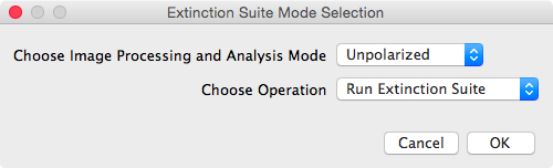 It then
prompts the user to select the processing mode, as unpolarized or
polarized (see panel shown to the right), and to select the
desired operation to execute. There are two operations
available: run the Extinction Suite, or run the folder mapping
module.
It then
prompts the user to select the processing mode, as unpolarized or
polarized (see panel shown to the right), and to select the
desired operation to execute. There are two operations
available: run the Extinction Suite, or run the folder mapping
module.
Mapping Module: Extinction Suite Folder Tree
The mapping module
creates the folder structure required by the main Extinction Suite
modules. It does not need to be run if you
are using stage-camera synchronous recording (see below).
This module is meant to support experimenters. Firstly, it
provides the structure which will be directly needed in order to
proceed with the extinction image development from raw acquired
data. Secondly, by immediately saving data into the appropriate
folders during experimentation, users can develop extinction
images for their present experiment "on-the-fly," allowing for
nearly-real-time evaluation of areas of interest. It is in
experimenters' best interest to make full use of this possibility.
The module will ask the user for a name (e.g. the date
"2015_01_01", 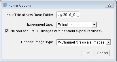 see
image at right), and create a folder of this name, which will
serve as base folder for the experiment and analysis. The
mapping of folders within the base folder differs depending on the
image data and processing mode for unpolarized or polarized
processing, whether or not extinction, extinction + darkfield, or
darkfield images are included, whether or not sensor offset
(background) images were taken at darkfield exposure settings, and
what kind of images will be recorded (M-channel greyscale images,
RAW, RGB, M-Channel Color). The latter option determines
what code path the converter and averaging modules will need to
follow. In the unpolarized case, within the base folder the
program will always create reference (R) and background (BG)
folders, while focus (F), dark-field (DF), and dark-field
background (DFBG), will be included depending on your choice
above. These folders have to contain the respective images
from your camera, regardless of image type.
see
image at right), and create a folder of this name, which will
serve as base folder for the experiment and analysis. The
mapping of folders within the base folder differs depending on the
image data and processing mode for unpolarized or polarized
processing, whether or not extinction, extinction + darkfield, or
darkfield images are included, whether or not sensor offset
(background) images were taken at darkfield exposure settings, and
what kind of images will be recorded (M-channel greyscale images,
RAW, RGB, M-Channel Color). The latter option determines
what code path the converter and averaging modules will need to
follow. In the unpolarized case, within the base folder the
program will always create reference (R) and background (BG)
folders, while focus (F), dark-field (DF), and dark-field
background (DFBG), will be included depending on your choice
above. These folders have to contain the respective images
from your camera, regardless of image type.
In case of single greyscale or composite input images,
acquired images should be saved directly to the appropriate
location, i.e. the F, R, BG, DF, or DFBG folders. Running
the main Extinction Modules, any images saved within these
folders will be moved into newly created subfolders named "RAW".
In case of multichannel data acquired via separate filters,
select "M-channel Greyscale images". Here, separate greycale
images or image stacks are required, with at least
one per channel per data type (F, R, etc.). Note, whether
or not the images are single files or stacks must be specified by
the user (see Input Image Options panel below) when running the
main modules of the suite. Stacks are recommended when possible.
An additional dialogue requests information on how many color
channels to use, and the names of the channels. For example "400,"
"500," and "600," indicating the center wavelength in nanometers
of the spectral range of the filter. The names must be given
comma-separated without spaces, so "400,500,600" in the example.
It is helpful if the names give the spectral information which
will be needed later on in the analysis section. Folders with
names given by the channels will be created in the R, BG, F, DF,
and DFBG folders. Acquired images should be saved directly into
their respective type and channel folders. For example, say a set
of 256 images were acquired as "focus" images at 500nm. The images
are subsequently saved as a stack, e.g. called "001.tif" or
"F_001.tif" in the location "BaseFolder/F/500/". Note, that there
is not an explicit restriction on the number of stacks that can be
saved in each folder. For example, say 2 sets of 128 images were
acquired as "focus" images at 500nm. The two sets of images
can be saved as two separate tiff stacks, e.g. called "F_001.tif"
and "F_002.tif", but must both be saved in the location
"BaseFolder/F/500/". The end result will be the same as saving a
single stack of 256 images. This possibility allows for more
complex referencing to be performed. For instance one can first
acquire and save 50% of the total focus images, then acquire and
save 100% of the reference images, then acquire and save the
remaining 50% of the total focus images. This is an example of
time-symmetric referencing and helps decrease the effect of
systematic drifts, e.g. lamp intensity/temperature, etc.
In case of multipolarization data ("Polarized" in option "Choose
Image Processing and Analysis Mode" seen above in the "Extinction
Suite Mode Selection" panel), the mapping is based upon the
polarization range of captured images (e.g. 0˚-180˚), and the step
size, in degrees. An additional dialogue requests the intial
angle, final angle and angle step size as integers. For each
polarization angle, a subfolder named as the angle value is
created in the base folder. For example for the angle range 0,
180, 60 , the subfolders 0, 60, 120, 180 are created. Each of
these contain the R, F, and DF folders. The BG and DFBG folders
stay in the base folder as the background is independent of
polarization. Folders related to the color channel will be
created in each of the available F, R, DF, BG, and DFBG folders,
if the user requires the M-channel greyscale
option, but not image conversion. Again, acquired images should be
saved directly into their respective polariser angle, data type,
and channel folders. For example, say a set of 256 images were
acquired as "focus" images at 500nm and \(0^\circ\). These data
are subsequently saved as a stack, e.g. called "F_500_000_001.tif"
or "001.tif", in the location "BaseFolder/000/F/500/". As in the
unpolarized case for M-channel grayscale images, multiple images
or image stacks taken for the same optical settings can be saved
to the same folder location to be processed together.
Note: the mapping module should be used
prior to acquiring the images, so that one can save acquired
images directly in the appropriate folders.
The folder structure is summarized in the table below
Unpolarized Analysis
|
Polarized Analysis
|
- Base Folder
- F
- e.g. 600 or R (if using color data w/out
conversion)
- e.g. 500 or G (...)
- e.g. 400 or B (...)
- D
- DF (if selected)
- BG
- DFBG (if selected)
|
- Base Folder
- First angle e.g. 0
- F
- e.g. 600 or R (if using color data w/out
conversion)
- e.g. 500 or G (...)
- e.g. 400 or B (...)
- ...
- D
- DF (if selected)
- Second angle, e.g. 60
- ...
- ...
- BG
- DFBG (if selected)
|
To run the module, choose "Run Folder Mapping Module" from
the operating mode drop-down menu (see Extinction Suite
panel).
Main Extinction Suite Modules: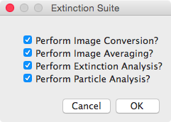
Choose "Run Extinction Suite" from the operating mode drop-down menu
(see Extinction
Suite Panel) to run the main modules of Extinction
suite. Ensure that you have captured all data required for
analysis (see Summary of Images to be
taken) and saved them in the correct folders in the folder
structure discussed above.
You will be prompted to select which modules may be run, see the
panel at the right. The modules can be run individually, or
in various combinations. Some require that the folder structure
contains the results of other modules. For instance, the
Particle Analysis requires that the results of the Extinction
Analysis.
After selecting ok, a dialogue requests a folder to be used as
the Base Folder for the analysis.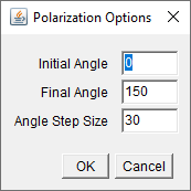
If the user initially selected "Polarized" from the initial
options panel (seen above in Initialization),
at this point they will be asked to define the first and final
positions of the polarizer in degrees, and the angle step size, as
seen in panel at right.
After selecting ok, a panel requests the main
characteristics of the data to be analysed. The content
depends on the module selection. The example panel, seen at
right, assumes that a converter or averager modules are
selected.
- Format of the captured images. Selecting the format
allows that the folders contain files other than those to be
analyzed, for instance ".rec" or ".txt" files containing camera
and image information recorded along with the image. Any
native formats of ImageJ, and any of the consumer RAW formats
listed on the Wikipedia
Raw Image Formats page are recognized.
- Measurement type (M-channel greyscale, RAW, RGB, or M-channel
color).
- Choose between single image or multi-image stack files.
(Instructions are given in the panel)
- Select to analyse extinction, darkfield + extinction, or
darkfield images.
- Enter comma-separated (no spaces) nominal center wavelengths
as integers of the spectral ranges used in your experiment. It
does not matter if there was only one dataset for one color
channel (spectral range) taken or if the image is RGB, you
must enter at least one value here.
- Method of darkfield background. The options are (A) no
darkfield background reduction (B) subtraction of DFBG images
(C) subtraction of a numerical offset.(Instructions are given in
the panel)
Converter Module: Conversion and RGB image channel splitting
This module is intended to convert RAW files, such as Canon .CR2,
to files usable by ImageJ, such as TIFF or JPEG. It can more
generally be used also as a batch converter between image
formats. The RAW files are opened with the DCRAW reader
plugin into 16-bit linear format for quantitative analysis.
For a detailed list of the image formats, which can be opened
using DCRAW reader, please see the DCRAW homepage
(toward the bottom).
The user selects which of the F, R, BG, etc. folders will be
considered for conversion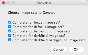 in the panel shown. ImageJ will determine the number of files in
the folder, and collect filenames from the folder in alphabetic
order. The averaging module, if selected, will create an
additional input panel.
in the panel shown. ImageJ will determine the number of files in
the folder, and collect filenames from the folder in alphabetic
order. The averaging module, if selected, will create an
additional input panel.
Next, if you are running only the converter module and
using colour images, you will be asked in the panel as shown if
you want to split the colour channels. 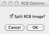 If yes, the split images will be created in subfolders called
"R","G", and "B" in each of the parent folders. If you selected
the averager module splitting is done by default.
If yes, the split images will be created in subfolders called
"R","G", and "B" in each of the parent folders. If you selected
the averager module splitting is done by default.
Next you will be asked if you used the mapping module to create
your folder tree. If yes, the program will use the related
folder names.  If
not, you will be asked to provide the title of the base folder and
the sub-folders in a panel as shown.
If
not, you will be asked to provide the title of the base folder and
the sub-folders in a panel as shown.
Next, if you run in "polarized" mode, you will be prompted to
input the Initial angle (0 default), final angle (150 default),
and angle step size (30 default), all integer, in degrees.
Next you will be asked in the panel shown for the destination format
and the range of images to convert, defined by the initial image
number, and the number of images. 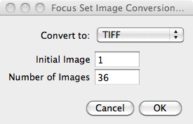 By
default the range is set to use all images in the folders. The
initial image and number of images to convert can be different
between the different kinds of images, i.e. Focus, Defocus,
etc. In polarized mode, the starting image and number of
images must be the same for all polarizations of a given image
kind. The panel shown refers to only focus selected, in
general these options are listed for each image kind selected.
By
default the range is set to use all images in the folders. The
initial image and number of images to convert can be different
between the different kinds of images, i.e. Focus, Defocus,
etc. In polarized mode, the starting image and number of
images must be the same for all polarizations of a given image
kind. The panel shown refers to only focus selected, in
general these options are listed for each image kind selected.
After this selection, the conversion will start. If RGB splitting is
chosen, the split images are stored in the R, G, and B
subfolders. If splitting is not chosen, or not possible, the
converted images will be created in a folder named "converted."
Averager Module: Image averaging
This module produces averaged images of all image files in each
subfolder; You are also given the option to create an RGB merged
average image, from the images in the R,G,B sub-folders assuming
an intially RGB or RAW image. The averaged images are stored in a
subfolder "Averages", with a identical R G B folder structure,
assuming a color image as input. If M-channel
greyscale images are averaged, then M averages are
created in the "Averages" folder for each of the image kind
folders.
In the option panels for the averaging modules (similar to the
one seen above for the conversion options), you will find a
checkbox option for deletion of individual converted channel
files. Check this if you want to delete the converted files,
hence saving space by keeping only the averaged, and original,
images.
You may use this module individually, in which case you will be
prompted to provide the folder names and the image format, as in
the converter module.
Extinction Module: Calculation of Extinction Image and
Dark-Field Image Preparation
This module assumes a folder structure as created by the
averaging module. It creates a folder in the base folder called
"Extinction" into which the processed images are saved.
- The extinction images are calculated as (1-(F-BG)/(R-BG)), and
are saved as 32bit float TIFF files.
- The dark-field images, are calculated as (DF-BG)/(R-BG), and
saved as 32bit TIFF files.
- All result images are stored in the sub-folder
"ProcessedImages" of the base folder.
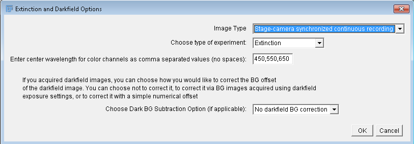
Extinction and darkfield options
In the panel at right, the main options of the extinction module can
be seen. Image Type specifies the format of the data, i.e.
"M-channel Grayscale", "RAW", "RGB", "M-channel Color", or
"Stage-camera synchronized continuous recording", which indicates to
the software what folder structure it should look for. Experiment
type can be "Extinction", "Extinction + Darkfield", or
"Darkfield". Color channel center wavelengths should be entered as
comma-separated values, no spaces, in the order the experiment
was performed. The final option defines how the
darkfield background should bee accounted for, including that it
should not be corrected. The latter should be used when no darkfield
data is present, and is the default option.
 This
module can be run separately. The script will search the folders
for the files to use. If no "Averages" exists, it will look for
"Converted". If no "Converted" exists, it will look for folders
matching the channel names earlier provided for the image kinds,
from which to take images. Failing that it will look for the same
number of images as the expected number of color channels directly
in the image kind folders. This is handy for "Extinction" image
processing.
This
module can be run separately. The script will search the folders
for the files to use. If no "Averages" exists, it will look for
"Converted". If no "Converted" exists, it will look for folders
matching the channel names earlier provided for the image kinds,
from which to take images. Failing that it will look for the same
number of images as the expected number of color channels directly
in the image kind folders. This is handy for "Extinction" image
processing.
Stage-camera synchronous recording
Available when neither converter nor averager are selected to run.
For experiments where stage and camera were synchronously triggered.
This is used for an improved version of shifted referencing
(discussed below), which reduces noise in the imaging arising due to
longterm fluctuations in the intensity or sensor. The sample
position is rapidly switched between two positions (shifts are
typically \(\ge2Ri\), discussed below). The camera records
continuously with images triggered via the MultiCARS software &
electronics also running the stage. After a preset number of images
taken at one position, the sample is moved with the camera still
recording. After a preset number of images at the second position,
the operation repeats. In our experimental setup, the sample
position moves in a rasterscan format without movement orthogonal to
the scan direction. In the example of a shift entirely in the
x-direction, the sample remains on the same vertical line. Hence,
one repetition is composed of positions x1, x2, x2
, x1, with n repetions. This is important, as in order to
process these into extinction images with the correct ordering, we
must know how many images are taken at each position, and how many
repetitions there are per channel. In this version of the code, we
assume a p1, p2, p2, p1 format of the repetitions. Therefore, for 4
repetitions of the scan with 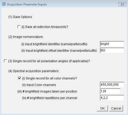 128 images
taken per position, with the total number of brightfield
acquisitions given by (4*128)*4=2048. Note, that this is not the
number of saved images. It is assumed the experimenter will
typically use online averaging (where possible) of images to
reduce the data storage cost, and that the averaging will be
equivalent to the number of acquistions per position. Hence, in
this example, assuming averaging of 128 acquisitions, there should
be 16 saved images. The user must indicate the number of
repetitions and the number of images averaged at each position.
Synchronous stage-camera single stack recording is flexible, and can
be expanded not just to take many repetitions of shifted
referencing, but also switching of color filter, or polarizer angle.
The user can indicate if this was done in the second panel (see
right). The options are to record as a single stack experiment per
polarizer per color channel (or vice versa), multiple stacks where
each stack is a single recording over polarizer angles, and with
each stack associated with a different color channel (or vice
versa), and lastly, multiple stacks where each stack corresponds to
one channel and one polarizer angle.
128 images
taken per position, with the total number of brightfield
acquisitions given by (4*128)*4=2048. Note, that this is not the
number of saved images. It is assumed the experimenter will
typically use online averaging (where possible) of images to
reduce the data storage cost, and that the averaging will be
equivalent to the number of acquistions per position. Hence, in
this example, assuming averaging of 128 acquisitions, there should
be 16 saved images. The user must indicate the number of
repetitions and the number of images averaged at each position.
Synchronous stage-camera single stack recording is flexible, and can
be expanded not just to take many repetitions of shifted
referencing, but also switching of color filter, or polarizer angle.
The user can indicate if this was done in the second panel (see
right). The options are to record as a single stack experiment per
polarizer per color channel (or vice versa), multiple stacks where
each stack is a single recording over polarizer angles, and with
each stack associated with a different color channel (or vice
versa), and lastly, multiple stacks where each stack corresponds to
one channel and one polarizer angle.
Files should be saved into a single base folder, named how the user
sees fit. Do not use the standard folder mapping. Files can be
titled however the user chooses in order to indicate background
(e.g. BG), or brightfield (e.g. bright), but if there are multiple
stacks, then the files must be titled with suffixes pertaining to
the separation of stacks. For instance, if there are 3 channels
(450, 500, 550), and 1 stack per channel, then the user should label
the brightfield stacks, (e.g.) bright_450, bright_500, and
bright_550. Or if there are 6 polarizer angles with 30 degree steps
starting from 0 degrees and one only channel, then the titles should
be bright_000, bright_030, ... etc. For multiple stacks with one
stack per angle per color, a double suffix should be used, e.g.
bright_450_000.
Background images need not be taken in the exact numbers as the
brightfield (darkfield) images. One background image per color
channel is required in order to account for the potentially
different exposure times. The background for each color
channel can be saved as a stack or can be pre-averaged by the user
and saved as a single image. In our current setup, it is not
possible to have different exposure times during a single
recording, so in this particular instance, you would only need one
background stack (or pre-averaged image) if you use single stack
recording over color, or single color and multiple stack
polarization recording. The single background stacks or
pre-averaged images in these cases can be copied and pasted into
the same folder with the appropriate suffixes added. Note,
background stacks will be averaged and subtracted as single images
from the brightfield or darkfield stacks, if the user did not
pre-average. Note that darkfield stacks can be recorded in similar
fashion using this continuous method, but without stage motion.
For more on the shifted reference technique see [PaynePRAP18].
Background images should be saved with the same nomenclature as
their brightfield counterparts (see paragraph above), and in the
same base folder location.
If no images are present in the offset folder identifier in the
prompt, a panel will request a constant value to be used as
background.
Note, for this method any acquired images including background
images, saved with the appropriate nomenclature as seen above, can
all be saved in the base folder. This compact save format was
chosen to compliment the compactness of this particular
experimental method. In-experiment, more rapid data acquisition,
and less navigation when saving images, decreasing time and focus
cost for the experimenter, as well as decreasing risk of saving
files in the wrong location. Hence, this method is particularly
handy when wanting to develop extinction images and examine areas
of interest on the fly during experiments.
Analysis Module: Particle analysis from Extinction Images and
Dark-Field Images
(A) Preliminary Options and Image Registration
This is a section with more significant input from the user,
however it has been streamlined and significantly improved from
earlier versions, reducing user input. The macro uses
ImageJ's built-in 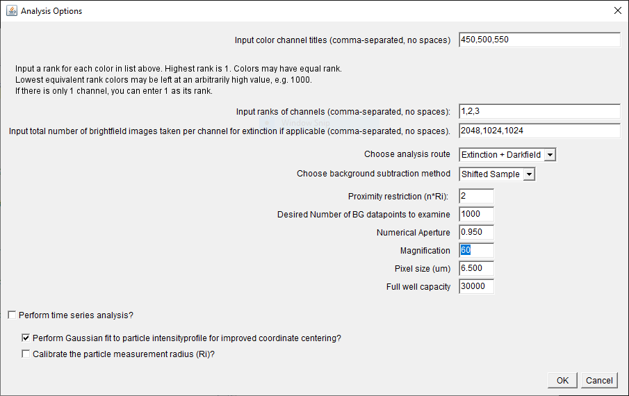 "Find Maxima" function to locate the
positions of the nanoparticles in the images. In order to do
this it must be thresholded appropriately above the image
noise. You will be prompted to choose the analysis options
after choosing a base directory if you did not already do this for
other modules.
"Find Maxima" function to locate the
positions of the nanoparticles in the images. In order to do
this it must be thresholded appropriately above the image
noise. You will be prompted to choose the analysis options
after choosing a base directory if you did not already do this for
other modules.
If you run only the analysis module (having perhaps
previously prepared the extinction images), you will see the
dialogue at right, the first option is to specify color channels,
again by center wavelength of spectral ranges. Only in the case of the extinction and analysis
modules the entries MUST be integers representative of
wavelengths in units of nm in the visible range (again
comma-separated no spaces).
The next option is quite important and serves as a general method
for spectral-filtering the results to select particles based on
spectral properties.
The color channels are ranked using positive
integers, with any two channels of different rank required to have
a lower cross-section in the higher rank channel. The lowest rank
image (minimum, 1) will be used to find maxima, and as the general
reference image throughout the analysis process. For
example, for channels (450nm, 500nm, 550nm), to filter results based
on the requirement that the cross-section, sigma, have the spectral
property sigma(450nm)>sigma(500nm) AND
sigma(450nm)>sigma(550nm), the ranks (1,2,2) would work. To apply
no spectral filter, choose ranks (1,1,1). Ranks must be input
comma-separated, no spaces. In
the case of the polarized analysis, the ranks are applied to the
polarization-averaged cross-section in each channel.
The next input is the total number of brightfield images taken
per channel. They are used to calculate the relative noise of
pixels in the image employed in the automated peak finding for the
shifted reference and drift calculations later. Again, entries are
listed in the order of the color channels, comma-separated, no
spaces. Note, that the total number of
brightfield images refers to the total number of Focus AND
Reference, inclusive of any averaging by the camera
prior to saving. Hence, if you averaged 128 Focus images, and
128 Reference images and repeated this n times, the
total number would be 2 x 128 x n. This
option will not appear if you have run the extinction module
immediately prior, as the values are defined in there.
If the analysis module is the only one selected, the analysis
route ("Extinction, "Extinction + Darkfield", "Darkfield") is also
requested. This will slightly alter options offered as the script
progresses.
The next option allows choice of two local background
subtraction methods, namely double radius, or shifted reference
method. Your choice here only applies to extinction images; the
double radius is always used when making measurments of scattering
cross-sections in darkfield. If double radius is chosen, for
extinction, the selection is based on your choice of experimental
acquisition of the reference image. In the publication, we use
only the 'defocus' reference method. However, for
high-sensitivity experiments, it may be more suitable to use a
'shifted' reference method. In this case, the reference
images are stored, named, and used exactly as the 'defocus'
(reference) images would be by the program. The difference
is in acquisition during the measurement period. If you
choose to use the shifted reference method, rather than
defocussing of the sample, please shift the sample laterally, via
stage controls, by a known amount of pixels. The shift can
be in the x or y directions, or in a combination of the x
and y directions. This shift will be automatically detected by the
software and provided to the user for optional adjustment; this
will be discussed further below.
The next option is the proximity restriction, removing particles
with a distance smaller than n*Ri. It
defaults to n=2 required to fit the Ri regions of the two
particles. It can be adjusted if required,
for example if the data were taken for the
shifted reference method with too small a shift.
The number of randomly chosen background points is next to be
adjusted. Any integer can be input, but typically this is kept
high for good statistical rigor.
The next 4 values are parameters of the optical setup: the
numerical aperture (NA), magnification (M), sensor pixel size (in
micrometers), and the full well capacity.
A checkbox is provided to enable time-series analysis of
extinction time-points. Note that data need not be actual
extinction data, but can be, for instance, fluorescence data. (see
section E below).
A checkbox is provided to enable Gaussian fitting of the peak
coordinates of all chosen particles, for improved measurement
accuracy. Fitting of coordinates is only performed after filtering
by proximity, cross-sectional range and the rank system discussed
above.
Calibrate the particle measurement radius (Ri)
To determine the optimum Ri, run the calibration. The
extinction image corresponding to the lowest rank channel will be
displayed. You will be prompted to locate a well isolated
particle, and to zoom in using the ImageJ toolbar. Place the
cursor on the center of the particle and then note the X & Y
coordinates shown in the ImageJ toolbar. Click "Ok" to close
the prompt. Enter the X&Y values in the next prompt amd
choose the maximum value of Ri over which to measure the
cross-section (default 100). A plot of extinction
cross-section versus measurement radius, Ri, is then calculated
and displayed. Inspect the plot and record the radius at which the
extinction cross-section saturates. This is your optimum Ri.
Close the plot. Typically, the saturation value foe matched NA of
objective and condenser 3 lambda / (2NA). We have recently
published a work which suggests this is a good nominal value.
Without running this calibration, the program will use this
formula as default the Ri for each center wavelength. For
more on the measurement radius see [PaynePRAP18, PayneSPIE19]. In
the Nikon Ti-U microscope stand with the Canon D-40 camera on the
left port with the sensor in the intermediate image plane, the
optimum measurement radius (3 lambda / (2NA)) is given by Ri=0.135
pixels*magnification*tube multiplier/numerical aperture. For
0.95NA 40x magnification with a 1.5x tube multiplier we find
Ri=8.5 pixels. In order to reduce noise for small particles, one
can choose a smaller Ri of 3 lambda / (4NA), which captures
still about 80% of the extinction, and post-correct the result to
represent 100%.
Additional options (for darkfield and polarization-resolved
cases)
Additional options are provided to the user after the initial
dialogue.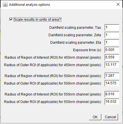
Via the tick box seen in the panel, one can choose whether or not
to scale the measurements in units of area, effectively
determining whether the output results are integrated pixel values
or cross-sectional values. This is a useful option for instance
when examining fluorescence data, which can be treated in the
software identically to extinction or darkfield data. Extinction
and scattering results would be typically be scaled, while
fluorescence would be unscaled.
If darkfield images are to be analysed, the scaling parameters,
tau, zeta, and eta are offered as inputs. The defaults are tau=1,
zeta=1, and eta=1, meaning the scattering results are unscaled. We
have the open-ended outlook that a code will be written to
calculate these parameters in the general dipole case.
Please see the above publications for more information; in
particular [ZilliPhD18].
The measurement radius, Ri will be calculated for each color
entered previously. These calculated values will be provided as
default. If the double radius local background subtraction was
selected, the double radius for each color channel is also offered
as input in this panel, and defaulted to 2Ri.
Using the double radius method, a particle must be spaced at
least 3 Ri from any other particle or debris, in order to avoid
overlap of the particle's local BG measurement between Ri and 2Ri
with the measurement region of radius Ri of other particles.
However, there might be other debris in the BG region, or we would
like to measure particles which are closer to each other. To
enable this, we can remove pixels in the BG region which are
outliers. In detail, we call the mean pixel value of the BG region
\(\Sigma\) their standard deviation
(called "sigma" in the user prompt). We then exclude any pixel
with a value more that
.
This is performed recursively, until no additional pixels are
excluded. N is requested in the "Additional analysis
option" panel (at right) when the defocus reference method is
chosen, and defaults to 2. In this way, we exclude points in
the BG ring, attributable to nearby particles/debris, so that a
particle distance of 2 Ri can be accurately analyzed, allowing for
increased particle density. If more than 50% of the
datapoints of the BG ring are removed by this procedure, the
particle is excluded from analysis. Choosing a large N,
say 1000, is effectively disabling the filter, if required.
(B) Maxima finding, shifted-reference and drift
automatic-registration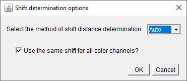
The shifted reference method results in the two appearances of
the same physical particle in the field of view of the extinction
image. The user will be prompted with two panels regarding the
magnitude (and direction) of the reference shift.
- The first asks (a) if the user wants either to run the
automated determination or to input the values for the shift
manually, and (b) if the user wants to use a single shift for
all channels (if there are multiple). Note the
auto-determination is carried out by a fixed-pattern
registration sub-routine written for this software. The shift
can be channel-dependent, but not polarization- dependent.
Experimentally, it is typically easiest to keep the shift the
same for all channels, but this is at the discretion of the
user. Likewise, it is more convenient in the analysis to use a
single shift for all channels (if this was the case
experimentally), because there are fewer values to enter, if the
user chooses to do so manually. If the automated routine is used
in conjunction with the single-shift option, the highest ranked
color channel is used to determine the shift, and this reference
shift is applied to the other channels. Note that for many
channels, this can result in a faster determination of the
shift.
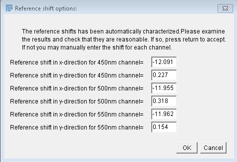
- The second asks the user to either confirm the values found
by the automated determination or enter the manual values they
have determined.
You will be asked to choose a regional ROI format and size. The
options for ROI shape are "Rectangle," or "Oval." Once selected, you
can adjust the ROI to desired dimensions. This can be used for
example to exclude regions where optical aberrations are apparent.
A screenshot after confirming the ROI shape and dimensions is
shown on the right. The prompt provides explicit
instructions. You start the "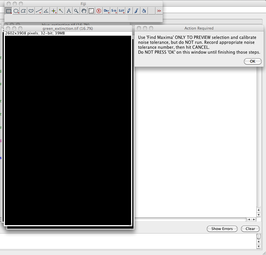 Find Maxima" protocol found in the ImageJ
Menu Bar->Process->Find Maxima. Since the extinction
images are normalized images, the threshold should correspond to
the relative intensity noise in the image, so in this example
0.0165. You can preview the number of maxima without running
the protocol (seen below). Do NOT actually run the protocol, and
do NOT press 'ok' on the above prompt until you have completed its
instructions. Brightness/contrast adjustment might be necessary to
evaluate the maxima which were found. A small fraction of maxima
which do not correspond to nanoparticles is acceptable. It
is important to choose the threshold close to the noise since the
background points used to determine the measurement noise are
taken outside a given radius around the maxima. After making
notation of the required noise tolerance, close the prompt,
leaving the extinction images as they are. This
Find Maxima" protocol found in the ImageJ
Menu Bar->Process->Find Maxima. Since the extinction
images are normalized images, the threshold should correspond to
the relative intensity noise in the image, so in this example
0.0165. You can preview the number of maxima without running
the protocol (seen below). Do NOT actually run the protocol, and
do NOT press 'ok' on the above prompt until you have completed its
instructions. Brightness/contrast adjustment might be necessary to
evaluate the maxima which were found. A small fraction of maxima
which do not correspond to nanoparticles is acceptable. It
is important to choose the threshold close to the noise since the
background points used to determine the measurement noise are
taken outside a given radius around the maxima. After making
notation of the required noise tolerance, close the prompt,
leaving the extinction images as they are. This 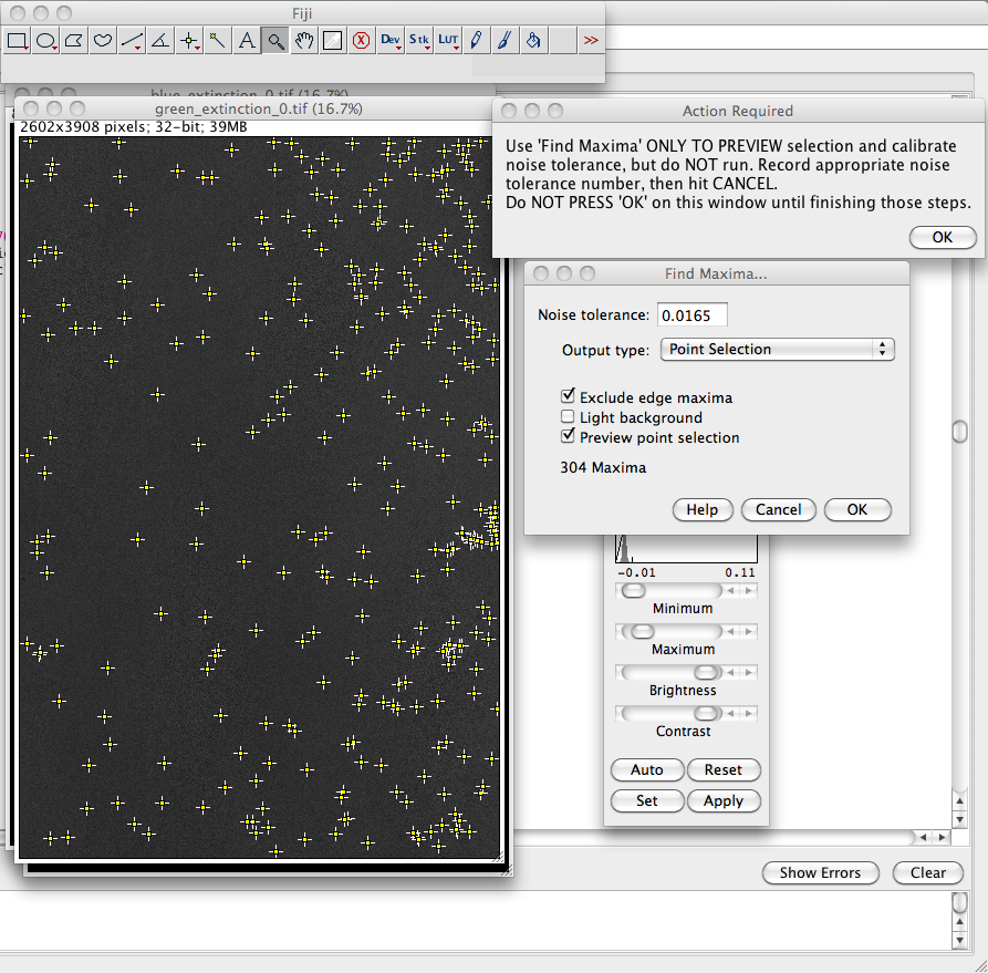 operation
is performed separately for extinction and darkfield images.
operation
is performed separately for extinction and darkfield images.
If you analyze dark-field images and extinction
images, analyze polarization-resolved images, analyze images for
different spectral filters, or any combination of these
experimental methods, it is common to see small transverse shifts
in the field of view due to drift or movement due to switching
from brightfield to darkfield, due to the rotation of the
polarizer, or due to filter switching. An image registration
(2D shift) can be applied to match the positions of the maxima
between each of the different cases. The registration proceeds
automatically via the same sub-routine as the shift-registration.
The algorithm used to register the images is based on pattern
recognition, specifically for N peaks found in an image, there are
N(N-1)/2 unique peak-pairs characterizing these N peaks.
Currently, the algorithm will initially search a small central
area of the image for N=9 peaks, and increase the search area in
the image either until it has found N=9 peaks (36 pairs), or until
it has reached the frame limits. It does this for each image and
then, roughly speaking, it compares each image to the first to try
to find as many matching pairs as possible. The shift is
determined as the mean distance (with sign indicating direction)
between the midpoints of the matching pairs of the two images.
When it cannot find any matching pairs, it will locate the two
closest peaks between the image to be registered and the initial
image, and determine the shift as the distance between these two.
When it cannot find any peaks in the images it will determine the
shift as zero in x and y. In both these instances, the user is
given the option to choose the shift manually.
In contrast to the shift determination, the drift registration
proceeds over potentially very different images and can be
susceptible to small issues raised by the automated peak finding.
This will likely not be a problem, however is largely untested in
darkfield. In general, you can assume it has worked if the shifts
seen in the panel to the right are small, or consistently
increasing. Sudden very large shifts (>30 pixels) instead
indicate errors in registration. To correct these, you can change
the noise tolerance to be more in line with the one you
established above. You can also adjust the "shift tolerance"
(default=0.5). These options are available after an initial
attempt by the software at registration if you choose to
re-register. Increasing the toleranc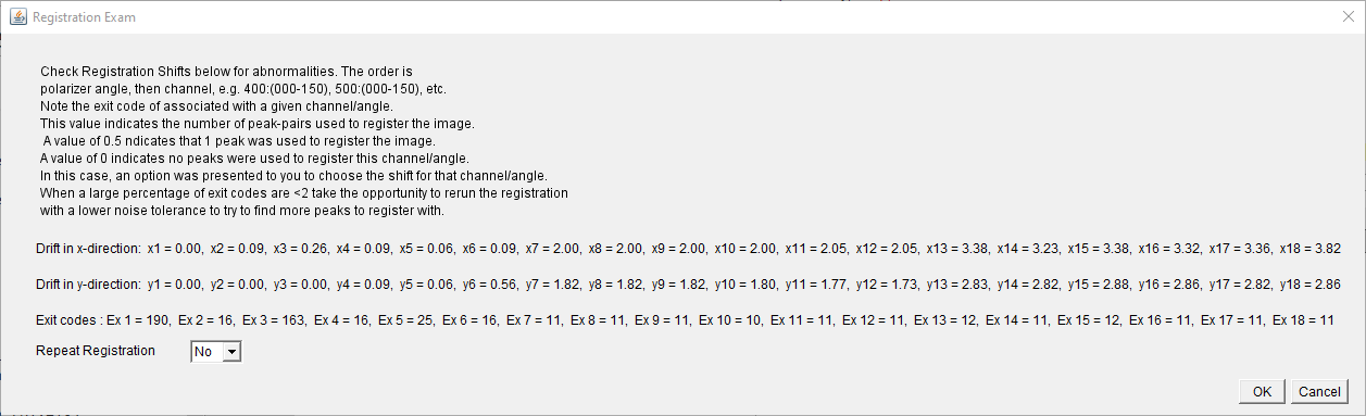 e can allow for some flex to
the pattern recognition. Decreasing the tolerance increases the
rigor of the pattern recognition. In the example of the panel,
shifts in the x-direction are smaller than 4 pixels in total over
the 18 image (3 channels x 6 angles) dataset, while y-direction
shifts are less than 3 pixels in total. Notice that shifts between
angles for a given channel (images 1-6, 7-12, 13-18) total less
than 0.5 pixels, while the shift observed when changing between
channels (6-7, 12-13) can be 1-2 pixels. Typical drifts are in the
order of 1 pixel per minute. We've seen up to a 25 pixel shift
between the intial and final extinction images over a 19 polarizer
angle experiment.
e can allow for some flex to
the pattern recognition. Decreasing the tolerance increases the
rigor of the pattern recognition. In the example of the panel,
shifts in the x-direction are smaller than 4 pixels in total over
the 18 image (3 channels x 6 angles) dataset, while y-direction
shifts are less than 3 pixels in total. Notice that shifts between
angles for a given channel (images 1-6, 7-12, 13-18) total less
than 0.5 pixels, while the shift observed when changing between
channels (6-7, 12-13) can be 1-2 pixels. Typical drifts are in the
order of 1 pixel per minute. We've seen up to a 25 pixel shift
between the intial and final extinction images over a 19 polarizer
angle experiment.
The exit code of the registration is output with the shift (see
panel) for the examination of the user before moving on from the
registration. The exit code corresponds to the number of pairs
used to register that image to the 1st image in the set. For
instance, if only one pair is used, the exit code is 1. If no
matching pairs can be found, the shift between the two closest
single peaks is provided. In this case the error code is 0.5. If
no individual peaks are found to register, the shift is taken to
be (0,0). The error code in this case is 0.
(C) Calibration 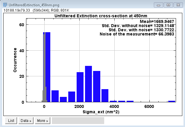
Next, the module will filter the maxima
which have a measured cross-section falling within a
user-selected range. The user selects this range by examining
the histogram of all particle cross-sections measured, where
particle locations correspond to those found by the find maxima
function previously. The histogram appears along with a
dialogue for the user. The histogram presents the both
the unfiltered particle data as well as the measurement noise for
the same color channel. The presented values are averaged over
all polarizations. The lowest ranked channel is the one used
for this data display. Likewise the color of the signal data (in
panel example here blue), corresponds to the wavelength of this
channel. A subroutine uses a custom color gamut to transfer
integer values of wavelength in the ~visible range (380nm-800nm)
to a hexadecimal color code. The dialogue offers the possibility
to re-display the s ame data with updated binning.
If you accept the binning (choose not to redisplay histogram via
"No" option), you will be provided with one more dialogue in which
to input the desired cross-sectional range. Particles with
cross-sections falling inside this range will be accepted.
Unfiltered particle data as well as this histogram will be saved
in the "Results" folder. Particles which fall within this
ame data with updated binning.
If you accept the binning (choose not to redisplay histogram via
"No" option), you will be provided with one more dialogue in which
to input the desired cross-sectional range. Particles with
cross-sections falling inside this range will be accepted.
Unfiltered particle data as well as this histogram will be saved
in the "Results" folder. Particles which fall within this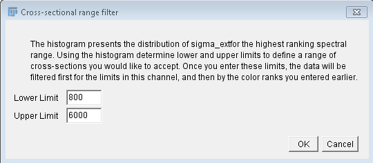 range will be further filtered by the rank
requirements discussed above.
range will be further filtered by the rank
requirements discussed above.
(C) Output Data
General
Analysis Metadata is printed in the ImageJ
Output Log and contains all user inputs to the
particle analysis. It is saved in the base directory at the
completion of analysis.
The final data will be saved in the form of excel files and
histograms, produced by custom scripting of ImageJ's plotting
capabilities. The histograms are saved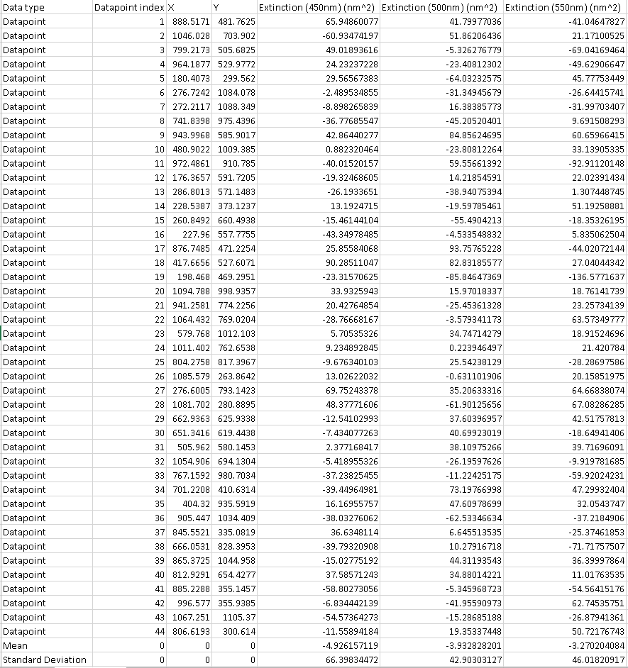 as .png images. A screenshot of a portion of the BG dataset
that would be output using the double radius method (specified at
the top of each column as DR-...) is shown. The actual
particle data is similarly presented. The data-type is given
in the 1st column ( datapoint, mean, or standard deviation).
The x and y coordinates of the BG points where the measurements
were taken are given in the 3rd and 4th columns. Notice that
the BG measurements are given in the form of a cross section and
were measured with the same radius, Ri, as the particles
were. To the right of the viewable region of that dataset
would be the scattering, similarly arranged. The amount of
resulting data will be accordingly large, particularly in the
polarized case. Histograms are provided for each color
channel. They show the distribution of cross-sections of the
BG and of the nanoparticles. Lastly, an extinction image is
saved, where each particle is labeled with its corresponding
number on the excel spreadsheet, making it easy to cross-reference
the data with the actual image. Polarization-averaged (or
unpolarized data) is saved either in the "Results" directory if in
unpolarized mode, or in the "RawStatistics" subfolder of "Results"
if in polarized mode.
as .png images. A screenshot of a portion of the BG dataset
that would be output using the double radius method (specified at
the top of each column as DR-...) is shown. The actual
particle data is similarly presented. The data-type is given
in the 1st column ( datapoint, mean, or standard deviation).
The x and y coordinates of the BG points where the measurements
were taken are given in the 3rd and 4th columns. Notice that
the BG measurements are given in the form of a cross section and
were measured with the same radius, Ri, as the particles
were. To the right of the viewable region of that dataset
would be the scattering, similarly arranged. The amount of
resulting data will be accordingly large, particularly in the
polarized case. Histograms are provided for each color
channel. They show the distribution of cross-sections of the
BG and of the nanoparticles. Lastly, an extinction image is
saved, where each particle is labeled with its corresponding
number on the excel spreadsheet, making it easy to cross-reference
the data with the actual image. Polarization-averaged (or
unpolarized data) is saved either in the "Results" directory if in
unpolarized mode, or in the "RawStatistics" subfolder of "Results"
if in polarized mode.
Polarized
In polarized mode, similar histograms are output also for each
color channel and each polarizer angle in a subfolder of the
"Results" folder called "PolarizationDependentFits," along with
polarization-dependence of the cross-section along with the fit of
this dependence (see paper), per particle per channel. This data
is saved as an excel spreadsheet in this same folder.
To simulate the noise in the measurement, a Monto-Carlo approach
is used. Adding to the data a random value from a gaussian
distribution of standard deviation given by the measurement noise,
and refitting a user-chosen number of times. In the subfolder of
"Results" called "FitStatistics" an excel spreadsheet of all
parameters of all simulated fits per particle per channel as well
as histograms of each of the particle's simulated fit parameters
are provided. Additionally the histograms of histograms for each
parameter is provided. Note that the contents of the
"PolarizationDependentFits" and "FitStatistics" folders are
subdivided into folders for each color channel if there are
multiple color channels worth of data.
(D) Automated re-analysis
If the user has need to rapidly re-analyze the same dataset, for
instance to observe the effect of varying values of a parameter,
e.g. Ri, one can utilize the automated re-analysis functionality.
To do this the user should run the Extinction Suite Particle
Analysis as they would normally do for a dataset choosing
parameters in the user prompts. We can call this run the Primary.
The output now includes text files in the “Processing” folder.
These are externally editable and the text has labels. 3 of these
are text files containing coordinates for peaks (or bg
datapoints). They are called by the program simply to know where
to make measurements.
The important file however for obtaining new results is the
“Parameters.txt” file. It saves all parameters in an ordered and
structured way so that Extinction Suite can read the file and load
the par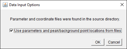 ameters. This file should be edited externally
with the new parameters of interest. To run the Extinction suite
on the same dataset with different parameters, one should make a
new base folder and put into it the “ProcessedImages" folder from
the Primary run. Additionally one should add a “Processing” folder
to this new base and into this place the .txt files from the
Primary run.
ameters. This file should be edited externally
with the new parameters of interest. To run the Extinction suite
on the same dataset with different parameters, one should make a
new base folder and put into it the “ProcessedImages" folder from
the Primary run. Additionally one should add a “Processing” folder
to this new base and into this place the .txt files from the
Primary run.
When running Extinction Suite particle analysis module, the
software checks to see if the “Processing” folder already exists,
and if a "Parameters.txt” is contained within. If so, a new prompt
is presented to the user requesting whether the user wishes to
load the parameters and coordinates from the files. Once the user
clicks yes, there is no more input from the user and Extinction
Suite will run at the exact same locations as in the reference and
with the exact same parameters from the text file, unless these
are externally altered.
(E) Time series analysis
Extinction and scattering time series naturally follow from the
experimental methods discussed in this page. Specifically,
stage-camera synchronous recording allows a variable
time-resolution method for obtaining time-dependent extinction
data, with resolution depending on choice of online averaging
number and acquisitions per position (discussed above in the
Extinction Module section). If observation of extinction as a
function of time is of interest, then one can run this part of the
analysis. However, other data which can be treated similarly with
respect to the analysis, such as time-resolved fluorescence data
can also be examined with Extinction Suite, and in particular
using this aspect of the software. Note, that output value scaling
can be the units of the area of the integral or can be unscaled
(see below in "Additional options").
Operations of Extinction suite vary only little compared to
standard, with an additional operation to choose a strong peak for
the time registration. Once registered, the time-sequence can be
averaged over a user-defined range, and then peak positions are
found, and proximity-filtered as in the normal analysis approach.
All proximity-filtered peaks are then filtered by their
area-integrated signal by the user. This filtering is performed
via a histogram presented to user by which they can judge and
define the max/min value range (as in the normal analysis
approach). After filtering, the average signal is measured for all
retained particles, then the time-dependent integrated signal is
measured (for all retained particles) and saved to an excel
spreadsheet. Particle data can be associated to the location in
the image in the typical way. The time-dependent signal of all
retained particles is plotted, and can be fitted with either
exponential decay (\(I=I_0\exp{-t/T}\)) or linear models. The fit
parameters are retained and recorded in the same spreadsheet that
the time-dependent signals are recorded.
Time-dependent data is saved in a subfolder of the Results
folder called "TimeDependentFits." Within "TimeDependentFits" are
subfolders called "Extinction_xxx_yyy" or "Scattering_xxx_yyy"
where xxx indicate the center (or otherwise descriptive)
wavelength of the filter range for the experiment and yyy
indicates the polariser angle. xxx will not be an empty
value, yyy can be empty and the preceeding underscore
removed, if the experiment was not polarisation-resolved. These
subfolders contain the above discussed data, fit paramters, and
plots associated with each wavelength and polariser angle.
In order to use this analysis section, one must of course have
time-dependent data. If developing extinction images using the
Extinction Module, one can choose to "Save all extinction
timepoints". Beware, this can result in significant data storage
cost if there are many images to be saved in an experiment and/or
many filters/polarisation experiments. The resulting time series
folders and images will be used directly in the time series
analysis. The nomenclature of the folders containing the timepoint
data is "Extinction_timepoints_xxx_yyy", where again xxx
and yyy have the typical meaning. If a user wants to
analyze darkfield (scattering) or fluorescence data, which may not
need explicit development like the extinction images, the user
should create folders of the above nomenclature in the base
folder, and place time series data into the folder named with the
appropriate wavelength/polariser angle. Note that if the data was
taken for unpolarized experiment type, then "_yyy" can be omitted
from the folder name. "_xxx" should never be omitted.
Summary of Images to be taken
The following images need to be
taken to determine extinction and scattering of a nanoparticle
sample
- Bright-field, ideally with an exposure time providing about
70% of the saturation counts of the camera
- in-focus
- out-of-focus, displacement about 10um (see [PayneAPL13]), or
alternatively for high sensitivity measurements
- a shifted reference image - an image of the laterally
shifted sample, with best results coming from a shift of ~2 Ri
[PaynePRAP18]
- Synchronously recorded stack where experiments for different
color channels or polarizer angles are saved as a single stack
or as multiple stacks.
- Dark-field images with suited exposure times. Dark field
intensities scale with the sixth power of the particle radius in
the dipole limit. A dynamic range of 1000 therefore corresponds
only to a factor 3 in radius. To increase the dynamic range you
can take two images with a factor of ~100 different exposure
times.
Last edited 03/11/2021
Wolfgang Langbein