Example of time-dependent analysis for widefield particle
extinction using Extinction Suite v4.1.5 or higher
- Unzip Data.zip
- "Data.zip" contains 1 folder: "TimeData". This folder will
act as the base directory for this analysis.
- "TimeData"contains 1 folder: "Extinction_timepoints_650".
This dataset was provided by Nicole Slesiona. The label includes
"Extinction..." as a requirement of the Suite in order to recognise
the folder structure, however the data is not made up of extinction
images. Instead it is a time-series of fluorescence data, each image
of which can be analysed in a similar way as typical extinction
data. The exposure time per frame was \(\tau=3\,\)s. The imaging was
performed with an objective of numerical aperture
\(\mathrm{NA}=1.4\) and magnification \(M=100\times\). The emission
wavelength is \(\lambda\sim650\,\)nm. The data has been
post-processed to remove hot pixels and background gradients, though
the specific methodology there is not important for the user to
understand. The data is ready to analyse as-is and serves only to
show how to run the time-dependent analysis and the kinds of results
one can expect.
It should be noted that the analysis operates in exactly the same
way whether one has time-dependent extinction or fluorescence data.
However, time-dependent extinction data can be obtained simply by
choosing to save all extinction timepoints when running the
"Extinction Analysis" module after having acquired shifted-reference
data using the stage-camera synchronous recording method. Note that
choosing to save all extinction timepoints results in an additional
folder containing the timepoints for each channel and polariser
angle in the experiment. In the case of the data above, we have only
one such folder, since the fluorescence was detected in only one
filter range (centered at \(\lambda=650\,\)nm. Here, the folder
containing the fluorescence data has been titled to mimic how the
folder would be titled if the suite was used to create timepoints
from extinction data.
1. Run ExtinctionSuite v4.1.5+
- Plugins \(\rightarrow\) ExtinctionSuite v4.1.5+
- Make sure no other images are open in ImageJ/Fiji, and then
close the welcome prompt.
2. Mode Selection
- Choose Unpolarised. Remember the primary dataset is
polarisation-resolved, but the secondary dataset is not.
- Choose Run Extinction Suite.
3. Module Selection
- Check "Perform Particle Analysis" only.
4. Choose Base Folder
- Navigate to the location of "TimeData"
- Select .../TimeData
5. Analysis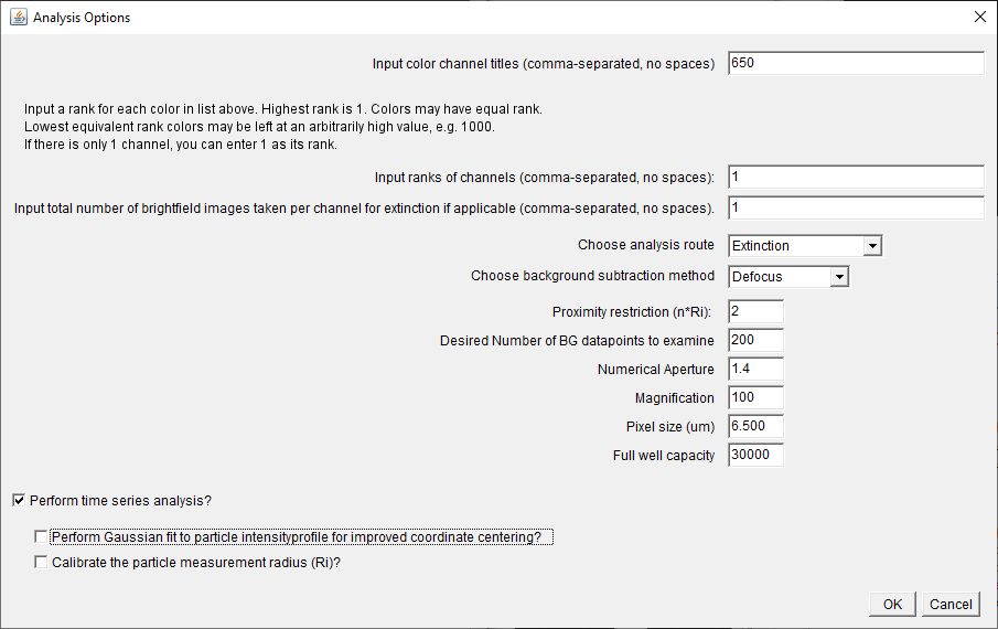
- Enter the values to match those displayed in the following
panel snip:
- Note that we choose rank 1 since there is only one "channel"
and 1 "brightfield" image acquired per channel. The latter is
only relevant when averaging data, where normally the
time-series are averaged to produce a single final image.
- In this case we select Extinction and the "Defocus" method.
The choice of "Defocus" is important here, since in
fluorescence data there are no bright-dark image pairs for
each object in the image as their are in shifted-reference
extinction data.
- Click ok on this first analysis panel and enter the values in
the next panel to match those seen in the following panel snip:
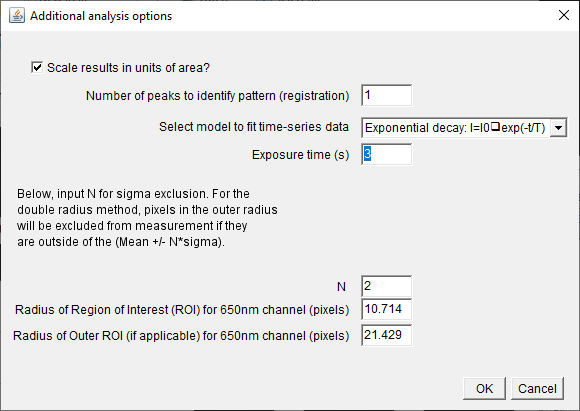
- The results can be scaled in units of area or unscaled at
the user's discretion.
- We will use only one peak in the image to register the
time-series.
- We select here the exponential decay model to fit the
time-series data.
- \(\tau=3\,\)s.
- Other items can be left as default, however if specific
local background subtraction considerations need to be made,
one can adjust the N-sigma value. In this example we choose
N=2.
- Select the peak shown in the screen snip seen.
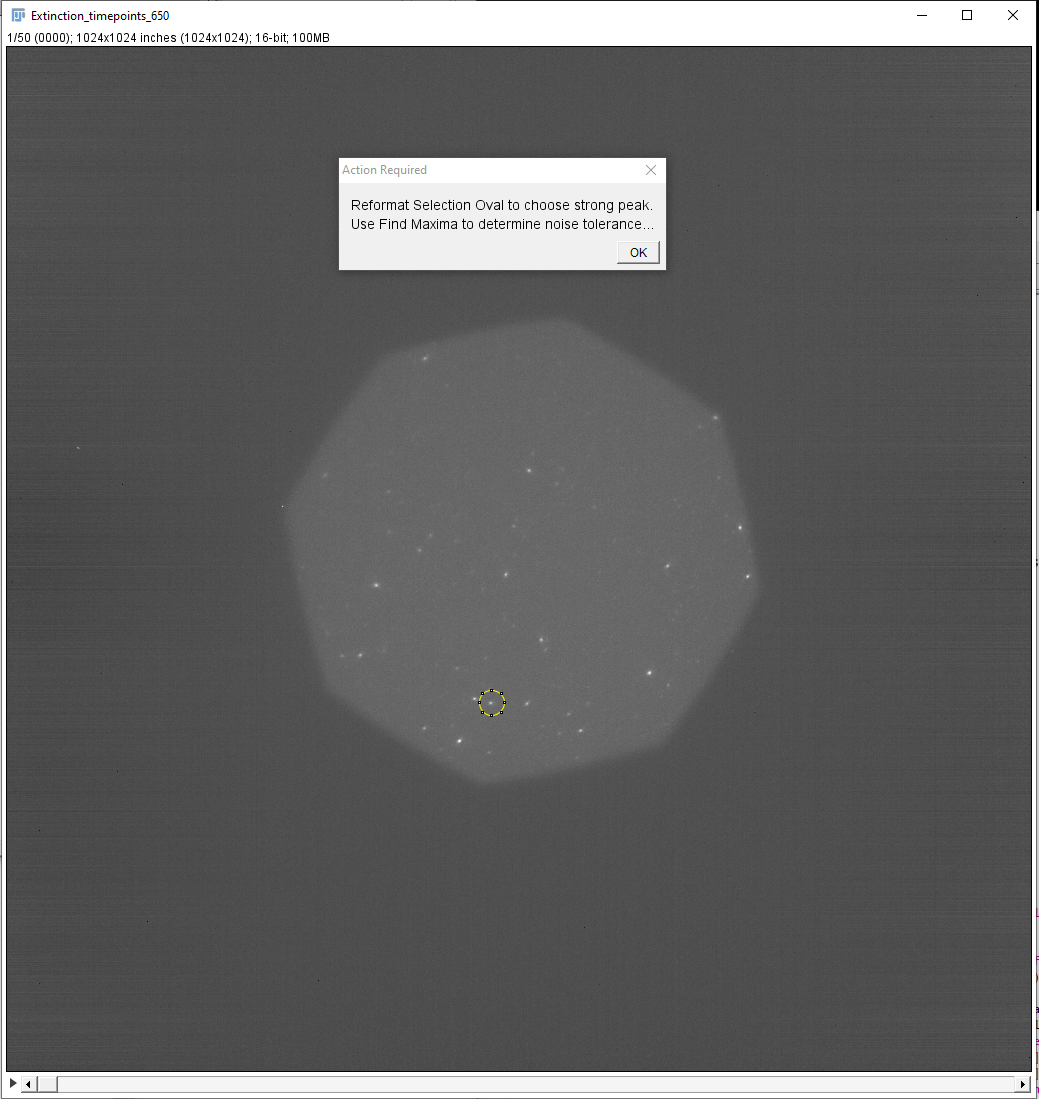
- You will need to reformat the selection oval to reject all
other peaks except the one desired.
- You should also run "Find Maxima..." to determine the best
noise tolerance to select one pixel in this peak. Do not click
ok until you have done this.
- In this case we find that a value of 200 works.
- Note that the entire time-series is visible via the scroll
bar at the bottom of the window during this time. Hence, you
can, in general, select which peak to use for the registration
by looking through the entire sequence and seeing which peak
is strong and visible throughout. Additional you can check the
noise tolerance at the beginning and end of the entire
sequence for this specific peak, to ensure that the value you
choose will select the peak even if its signal diminishes over
time.
- Enter the values in the Registration Options panel to match
those seen in the panel snip:
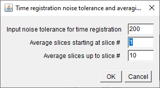
- As mentioned in the previous point, we found a value of 200
works for the noise tolerance to find the max pixel of the
selected peak over the entire duration of the series.
- The averaging range here is important.
- The averaging performed here will be used to create an
averaged image with which one will select as many peaks as
possible for which to acquire measurements.
- In this example, only 50 frames are provided, however the
series could be hundreds or more frames long.
- It's important to choose enough frames to average that we
can see peaks more clearly above the noise for the purposes
of peak finding, but not to select too many so that peaks
whose signal decreases quickly after the beginning of the
frame are averaged away.
- Here we choose to average the first 10 frames.
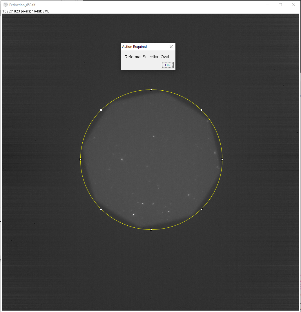
- Click ok and then choose to use an Oval format ROI.
- Reformat the oval to approximately match that of the screen
snip, then click ok.
- You will be presented with a panel indicating you should once
again use "Find Maxima.." to determine a noise tolerance to use
to select as many peaks in the image as possible to measure. We
have found that a value of 30 here selects most of the visible
peaks.
- Note that in this case we are choosing our noise tolerance
using the averaged image.
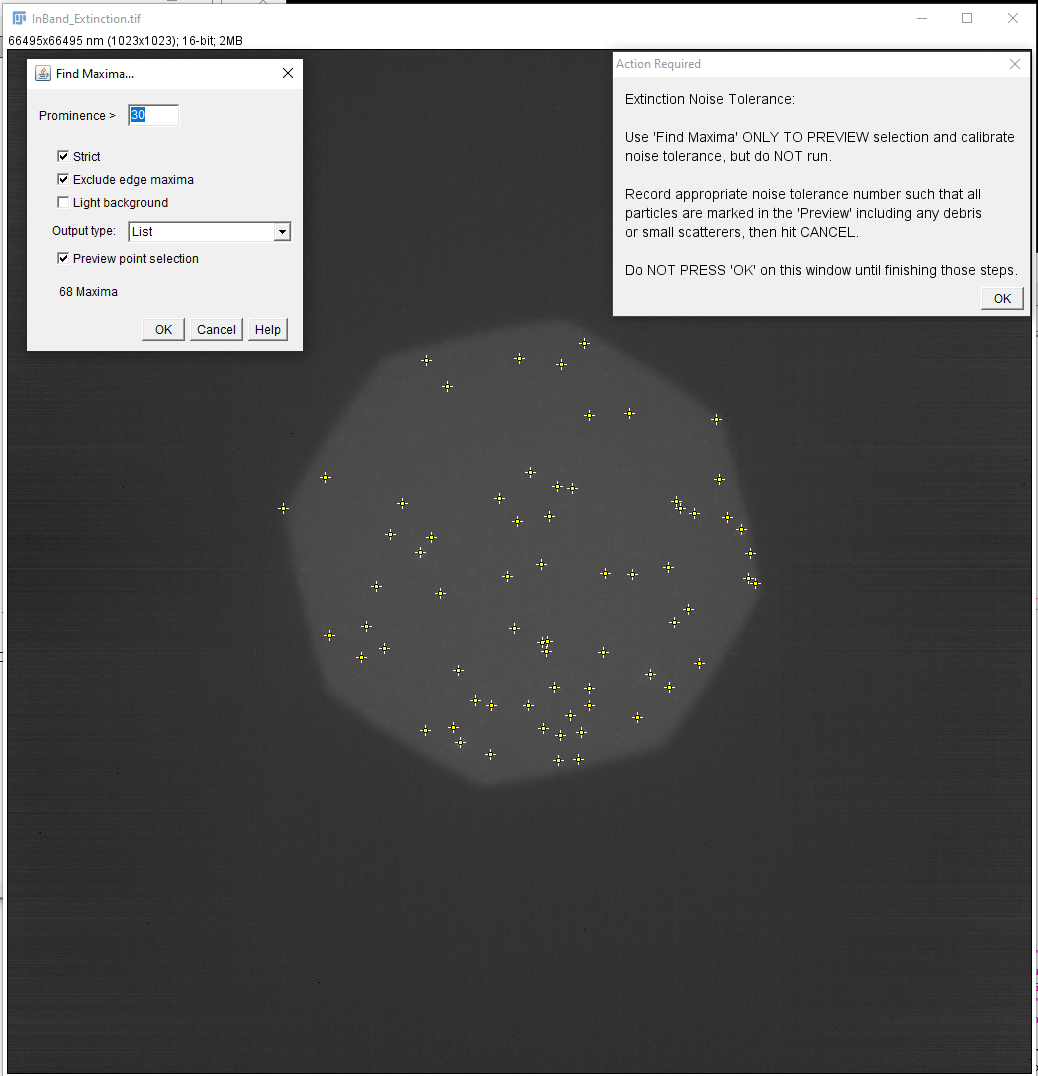 Click ok on the
instruction panel and the data will then be analysed.
Click ok on the
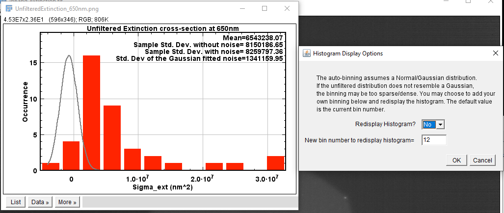
instruction panel and the data will then be analysed.- Once the initial analysis operation finishes, you will be
provided with the statistics of the results (integrated
intensities) obtained by measurements of individual peaks in the
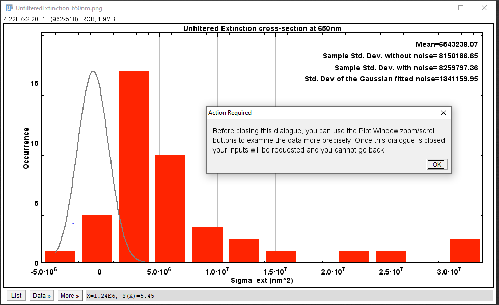
averaged image. If you wish you can redisplay the histogram with
more or fewer bins as seen in the screen snip:

- In order to move on, choose NO to skip histogram re-display,
and then select the data range to filter the peaks you wish to
analyse for their time-dependence. We have chosen in this
example to exclude all data below approximately one standard
deviation of the noise (gray line Gaussian curve), i.e. we
exclude \(\sigma<\sigma_\mathrm{noise}\). Hence, the lower
bound of our selection is 1000000. We will keep all data above
this, and choose the upper bound to be 32000000. Click ok.

- The analysis will proceed and you will be informed when it is
complete.
- This completes the time-dependent analysis tutorial.
- Please examine the content of "Results" folder.
Created by Lukas Payne, 18/09/2021, edited
19/09/2021 WL.


 Click ok on the
instruction panel and the data will then be analysed.