
Dirt filter specific controls in the qDIC software.
The program qDICv320.exe
is used to integrate the quantitative differential interference
contrast microscopy (qDIC) images. It reads raw DIC images and
performs an DIC inverse transformation using a procedure based on
Wiener deconvolution, and saves the calculated differential phase
(delta) and integrated phase (phi) as tiff, ascii and matlab
binary files. You can run the executable qDICv320.exe directly, or the batch
file qDICv320.bat
to provide a command line window where matlab errors during
execution are displayed.
See the publication [1] DOI
10.1016/j.bpj.2013.07.048 for more details of the underlying
science.
See an example of
qDIC measurements of grooves in photolithographic polymer SU-8
(unpublished) [2].
This program is written in MATLAB R2021a. It is a stand-alone application, so it does not require a full MATLAB installation. The program has been tested under Windows 10 Pro, Intel i5-2400 processor @3.10 GHz and 20 GB of RAM. It is necessary that the MATLAB Compiler Runtime (MCR) version 9.10 (R2021a) is installed. If the MCR is not installed, do the following:
DIC is a measure of the phase difference between two adjacent
points in the sample plane. The exact Fourier multiplier of the
DIC-like transformation is given in [1], formula (6). The inverse
transformation is done using Wiener deconvolution, see [1],
supporting material, formula (4). Depending on the assumed
signal-to-noise ratio, κ, the result changes, as
effectively a high-pass filter is applied to the data in the shear
direction: For low κ the integrated images show less
integration artefacts and less long-range features, such as phase
steps. High κ allows the recovery of the long-range
features at the expense of noise related stripes along the shear
vector direction.
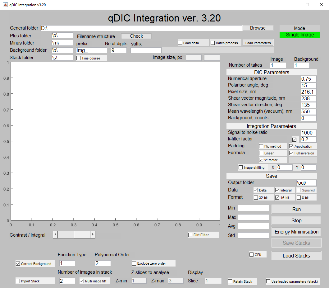
The user needs to specify the location of data files on the hard disk (general folder). Within that folder, the user should create subfolders, "p" and "m", which contain the raw DIC images taken for positive and negative ellipticity of the incident beam respectively. The absolute value of the incident ellipticity for positive and negative phase should be equal; if not the polariser may not have been calibrated correctly during imaging. The filenames are constructed using the default settings of the Hamamatsu camera software. The variable part between prefix and suffix has a fixed number of digits (9 in this case), so the files are img_000000000.tif, img_000000001.tif, etc. The user can browse for data folder using "Browse" button, and can check the filename using "Check" button. Note that the prefix, the number of digits and the suffix are all modifiable so that the user may use their own image naming convention (this must contain digits however).
Usually, several acquisitions of each field of view are taken and averaged together. If these have not been averaged before loading into the qDIC software, the number of acquisitions (1 by default for DIC images) should be specified. These acquisitions are then averaged by the qDIC software before further processing.
The user should take background images in order to subtract the dark counts from the DIC images (these should be stored in a subfolder "b"). As in the case of the positive and negative images, multiple repeats may be taken. If these are not averaged together before running the software, the number of frames should be entered in the "Background" box. Alternatively the user may measure the average dark counts (plus leakage) value throughout the image and input it in "Background, counts" field under the DIC Parameters heading. An error message will appear if no background images are found; the program will still run and use the average dark counts instead. It is not advisable to use both methods of background subtraction at once, which is why the "Background, counts" field is set to 0 by default. If no background images are used, set the "Background" field to 1 (default).
The user can place single multi-image *.tiff files in the \p\
and \m\ folders, and tick the "Multi image tiff" checkbox and
input the filename in the manner described above (Files and
folders for single z-planes). To import stacks, tick the box
"Import Stack". The tickbox "Retain stack" is automatically
activated in stack mode upon hitting run to avoid the re-import of
the stack and calculation of the differential phase data.
The user may also create a stack of integrated images through
placing multiple *.tiff images in the \p\ and \m\ folders and
unticking the "Multi image tiff" checkbox before hitting "Run".
The variable part between the prefix and the suffix changes in
a manner described in the section above when the software reads in
file names, however the number of images which are read in is
limited by the "Number of images in stack" field rather than the
"Number of takes" field.
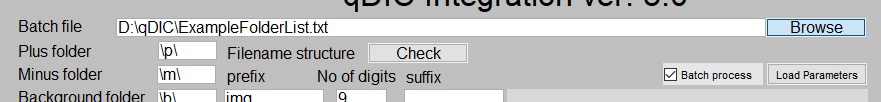
To facilitate the analysis of large numbers of data sets with the
same parameters, the batch processing option is available. To use
it, first check the "Batch process" checkbox. Note that the label
for the directory textbox will change from "General folder" to
"Batch file", and the "Run" button will change to "Run batch" to
indicate the change in mode.
Next, a *.txt file must be created with a list of folders to be
used for the analysis. An example of this is shown below.
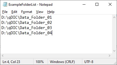
Each of the folders listed in the text file must follow the
standard structure, with subfolders for the positive, negative and
background images (named "p", "m", and "b" by default) and files
named according to the naming system entered into the software.
Next, enter the file path for the file containing the folder list
into the qDIC software.
Once this is done, the integration parameters are entered the same way as when processing a single data set, outlined in the sections below. Note that the software will use the same analysis parameters for every data set on the list; if some data requires different settings, these should be split into separate files. Once the correct parameters have been entered, click "Run batch". The software will then process the data in each folder on the list sequentially.
An option exists to integrate a differential phase (delta) image
directly, rather than first generating the differential phase
image from a pair of positive and negative DIC images, and then
integrating. This mode is activated by checking the "Load delta"
checkbox. These delta images should be in the "out" subfolder,
named delta.mat, and be formatted to match the qDIC software
output, with the name of the differential phase variable in the
.mat file set to "delta_out".
In this section, the user needs to enter the settings relating to
the acquisition of the DIC images during the original measurements
session. Specifically, this includes the numerical aperture of the
system (usually equal to the numerical aperture of the objective),
the polariser angle used, the pixel size (determined by the
objective, tube lens, and camera used), the size of the DIC shear
vector, the direction of the DIC shear, the mean illumination
wavelength, and the background counts (only needed if a background
image is not used). Information on the pixel size for different
objective and tube lens combinations is available for the Ettore
and Galileo
microscopes. Measured DIC shear vectors for N2 and NR DIC prisms
are available here.
The signal-to-noise ratio of the Wiener deconvolution determines the low spatial frequency cut-off of the reconstruction. The user should look at the resulting integrated images and see if the degree of noise is tolerable. The value of 4000 was found to be a good trade-off for the Galileo microscope and the 0.75NA objective with 1.5× multiplier.
Spatial frequencies that are above the Nyquist limit of the
optical setup can be filtered out using the k-filter - a cosine
apodisation from 1 to 0 is used to smoothly reduce the Fourier
amplitudes for spatial frequencies above the k-max value to zero
(k-max is the Nyquist limit of the optical system). The k-filter
factor defines the range of spatial frequencies over which the
apodisation function is used. The size of this range is determined
through multiplying the k-filter factor with k-max. NOTE: k-max is
the central value of the user defined range over which the
apodisation function is used, so values above and below k-max are
apodised and some spatial frequencies above k-max will have a
non-zero amplitude. There is a checkbox to enable this feature and
it is used by default.
This function can also be used to suppress the data at spatial frequencies corresponding to the inverse of the DIC shear, which leads to increase in noise with a period of the sheer. For this goal, the NA setting has to be set lower so that the spatial resolution \(\lambda/(2\mathrm{NA})\) is above the shear. For the N2 DIC slider shear of 238nm, and 550nm wavelength, this requires setting the NA to 1.1 or lower at a filter factor of 0.1 or lower.
In order to reduce artefacts in the integrated images caused by
the periodicity of the Fourier transform, the software offers two
methods of padding the data prior to the integration.
In either case, the padded area is automatically cropped out
following integration.
This option allows the user to use a linearised version of the equation for extracting differential phase from the composite DIC image as opposed to the fully invertible equation (full inversion is recommended by default, see qDIC example for details).
This is a checkbox which is used to make the mean values of the
background subtracted positive and negative polarisation DIC
images equal through multiplying both images by a factor. This
checkbox is checked as default and it compensates to first-order
different mean values of positive and negative polarisation DIC
images due to inaccurate phase offset settings and setup drifts.
The program saves all resulting files in the subfolder with name
given by the "Output folder" field within the "General folder".
Multiple runs of the program in single image mode will overwrite
the previous version of the files, so it is recommended to copy
them elsewhere or to change the "Output folder" location.
The user can choose to save differential phase delta and/or
integrated phase phi. For each phase, three files are saved: a
tiff image (in either 8, 16, or 32-bit format), a *.dat file
(ascii), and a *.mat file (binary Matlab format). All files
contain absolute values of the phase in radians, unless either the
8 or 16-bit checkbox is checked then the tiff image is in unsigned
8 or 16-bit format respectively. However, this can be scaled using
the min/max values in the metadata under the 'ImageDescription'
tag.
If the "Import stack" tick box is unchecked, the contrast and integrated images are saved automatically after processing (as in previous versions).
Stacks are saved as 8/16/32-bit multipage tiff format after
analysing stacks and hitting the "Save button" (stacks will not be
saved otherwise!). In addition to the option to save the
differential phase delta and integrated phase phi, an option to
save the squared image is also available for stacks. If z-planes
are not integrated, they are not saved within the outputted
contrast/integral/squared images. A string of data is saved along
with the image stacks (one each for phase, contrast and squared
images) that indicates the length of the original image stack, and
the integrated images - for example if the 2nd z-plane is
integrated, a value of 1 is recorded at position 2 within the
string, if it remains unintegrated a value of 0 is recorded at
position 2 within the string. This string of data also "inflates"
the z stack to its proper size upon reloading the data in qDIC.
The parameters used in for each z-plane are saved in a *.mat file named "Stack_parameters.mat" upon hitting the "Save Stacks" button.
Single images / image stacks can be saved in either 8-bit,
16-bit, or 32-bit format by using the checkboxes under the "Save"
heading. Using 16-bit format approximately halves the data size
relative to 32-bit, and using 8-bit halves it again. For 8 or
16-bit images, the minimum and maximum values are saved in the
metadata of the TIFF files under the metadata Tag
"ImageDescription".
An ImageJ/Fiji macro to automatically read this information and
apply the correct intensity scaling, PixelCalibration_v2.ijm, has
been developed by Lukas Payne, and is available here. Note however that this
calibration method (using the built-in "Calibrate" tool in
ImageJ/Fiji) is not compatible with hyperstacks; concatenating
stacks into a hyperstack changes the intensity calibration to
incorrect values.
This feature corrects slowly varying background changes (often seen in the direction of the shear vector), and is activated by a tick box named "Correct Background".
Small, high contrast objects in the DIC images can cause
significant artefacts in the integrated image, along the shear
direction, particularly at high values of the signal-to-noise
integration parameter. Such artefacts may interfere with
measurements elsewhere in the image, and so it is sometimes
desirable to remove such objects. The dirt filter allows the user
to manually select regions of the image containing unwanted
structures, and replace them with a region that is mostly smooth
and featureless (a similar procedure as the apodisation is used,
see PhD of J.B.Williams) which should not produce significant
artefacts.
Dirt filter specific controls in the qDIC
software.
To use the dirt filter, check the "Dirt filter" checkbox before
clicking "Run". When the dirt filter is checked, a number of
additional buttons, textboxes and checkboxes will appear which
control the functions related to the dirt filter; these are shown
in the figure above. Once the user clicks "Run", these buttons
will become enabled, and, after the polynomial background
correction is complete, the processing of the image will pause to
allow the user to filter the image as desired.
To apply a filter to a region, draw a rectangle on the image,
adjust it as desired, and then click "Apply Filter". The image
will be updated immediately to show the image after filtering, and
the number displayed in the "Total Filters" box will increase by
one. To undo one of the filters applied to the image, use the
"Filter No" textbox to select a previous filter and click the
"Delete Filter" button. The corresponding filtered region will
then have its original values restored, and the index of the
filters of higher number will be reduced by one.
To facilitate the application of the filters, zoom and contrast
adjustment options are available. To use the zoom, simply use the
rectangular selection to select a region of the image to zoom in
to and click the "Zoom In" button. To cycle between several
enhanced contrast presets, click "Contrast". The "Zoom Out" button
restores the full field of view.
When using the dirt filter with stacks, the user will be
presented with a prompt asking if the user wants to use the same
filter regions on each frame:
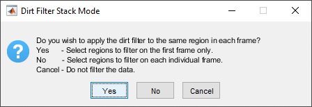
If the user clicks "Yes", the user will be allowed to select any number of regions to filter on the first frame, and then these same regions will be automatically filtered on all subsequent frames in the stack. If the user clicks "No", the user will be allowed to select different regions to filter for each individual frame in the stack.
The qDIC software has two methods of loading in integration
parameters:
When carrying out any integration on a single frame image, or saving the results of an integration on an image stack, the saved .mat files include a variable called "Metadata" which records every setting of the qDIC software when the integration was carried out. Each time the analysis is rerun or a stack is saved, the settings stored in the .mat data files are overwritten. However, each time the analysis is run, a separate .mat file is also created named with the name format settings_YYMMDD_hhmm.mat, where YYMMDD_hhmm refers to the date and time the analysis was run, so previously used settings can still be accessed and reapplied.
To load in settings used for any previous analysis, click the "Load Parameters" button located under the "Browse" button near the top right of the GUI. Click any file (either a settings file, or a delta or phi .mat file) to load in the settings stored in that file.
A previously implemented system for loading parameters that only works on stacks is the "Use loaded parameters (stack)" checkbox. This function uses the "Stack_parameters.mat" file that is saved alongside stacks, and differs from the "Load Parameters" button in its ability to apply different settings to each slice of a stack. This may be useful when trying to test different integration parameters, or if the imaging parameters changed between frames.
This mode is used by just ticking the "Use loaded parameters (stack)" checkbox, and hitting "Run". NOTE: to use parameters saved from previous session on a stack that has not yet been analysed, place a copy of the "Stack_parameters.mat" in a folder named "out" (if the default value for "in folder" is unchanged) - place this folder in the same directory as the "p", "m" and "b" files.
To run the program on a stack of images, check the "Import Stack"
checkbox. The software has two modes for handling stacks.
The default method takes a stack of N positive
polarisation images from the "p" folder (still named according to
the system described above, so img_000000000.tif by default), and
a corresponding stack of N negative polarisation images
from the "m" folder, and will then run through all the frames in
these stacks, taking the ith positive image and the ith
negative image and generating delta and phi images from them in
the same way as for single image mode, ultimately producing output
delta and phi stacks with N frames.
The software can also be used to integrate stacks taken at a
single polarisation, such as time course measurements or z-stacks.
This analysis mode is enabled by checking the "Time course"
checkbox in the top left region of the GUI. Time course data will
consist of a stack of consecutive images taken at the same
polariser angle +φ, and two reference single-frame images
taken at +φ and -φ, named I+
and I-, while z-stack data will consist only of
a stack taken at a single polarisation at different z-planes. Note
that the time course or z-stack *.tif file should be placed in a
subfolder named "s" and named according to the standard format.
For the time course, the I+ and I-
images should be saved in folders "p" and "m" as usual in the
general folder.
There are three options for calculating the contrast image. When
the user runs the analysis with the time course option checked,
they will be asked to choose between these three settings from a
dialogue box.
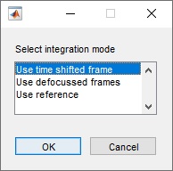
In the first option, designed for time course data, a time
shifted image is subtracted from each frame, as described in the
equation below: $$I_c=\frac{2(I_{n+\Delta}-I_n)}{I_+ + I_-}$$
where Ic is the contrast image, In
is the nth image in the time course, \(\Delta\) is a user defined
number of images for the time shift, and I+ and
I- are the positive and negative reference
images respectively.
The second option is designed for analysing single polarisation
z-stacks. This option uses two frames shifted from the focal plane
by a set amount for referencing. The contrast image for each
slice, z is given by: $$I_c = \frac{4I_{z} -
2(I_{z+\Delta} + I_{z-\Delta})}{2I_{z} + I_{z+\Delta} +
I_{z-\Delta}}$$ where again Ic is the contrast
image, Iz is the image at focal plane z,
and Δ is the user defined number of frames to shift by in
the analysis. Note that unlike the other referencing options in
the software, this analysis mode does not require anything in the
"p" or "m" folders; only the stack (and background) is needed. The
stack may be taken at either positive or negative orientation.
When the third option is selected, a positive reference is
subtracted from each frame instead, as in the following equation:
$$I_c=\frac{2(I_n-I_+)}{I_+ + I_-}$$In each case, the background
image is subtracted from all images I before the contrast
image is generated.
This checkbox allows the user to retain contrast/integrated
images and integration parameters used within a stack for the
current session. If the user needs to clear these images, this
checkbox should be unchecked.
This button will load integrated stacks from a previous session.
The stack parameters will also be loaded (if a
'Stack_parameters.mat' file is present) and will be present upon
changing the Z-number display parameter.
The user can specify which z-planes within the stack are to be
analysed through using the "Z-min" and "Z-max" fields. Through
this function, the user can integrate each (or multiple images)
with a particular set of integration parameters.
The energy minimisation panel appears, and the user can load a "delta" and "phi" image through a browse button. The pixel size, shear direction and shear magnitude fields are filled with the same values as those that are in the main qDIC window, but can be changed by the user.
GPU mode can now be used for energy minimisation on computers
with suitable graphics cards. The GPU option is automatically
enabled if a suitable GPU can be used. In the GPU mode, a range of
smoothing factors between \(10^{-{q_{min}}}\) and
\(10^{-{q_{max}}}\) can be tested. The smoothing factors
\(S=10^{-q}\) are generated using the set of integers
\(q=\{q_{min},q_{min}+1,\ldots,q_{max}-1,q_{max}\}\), where
\(q_{min},q_{max}\in \mathbb{Z}\) and
\(0<q_{min}<q_{max}\). DIC images can be loaded after
integrating single plane images and loading the *.mat files into
the Energy minimisation software. *.tif images can also be used.
If using the GPU mode for high speed computation, images should
not be displayed frequently, as gathering the image from the GPU
and displaying these images in the panel is a slow process.