The program qDICv222.exe is used to
integrate the quantitative differential interference contrast
microscopy (qDIC) images. It reads raw DIC images and performs DIC
inverse transformation using Wiener deconvolution principle, and
saves the differential phase delta and integrated phase phi as
tiff, ascii and matlab binary files.
This program is written in MATLAB R2015a. It is a stand-alone application, so it does not require a full MATLAB installation. The program has been tested under Windows 7 Enterprise 64-bit, Service Pack 1, Intel i5 processor @3.10 GHz and 20 GB of RAM. It is necessary that the MATLAB Compiler Runtime (MCR); version 8.5 (R2015a) is installed. If the MCR is not installed, do the following:
DIC is a measure of the phase difference between two adjacent points in the sample plane. The exact Fourier multiplier of the DIC-like transformation is given in [1], formula (6). The inverse transformation is done using Wiener deconvolution, see [1], supporting material, formula (4). Depending on the assumed signal-to-noise ratio, the result is changing, as effectively a high-pass filter is applied to the data in the shear direction: For low s/n the integrated images show less of integration artifacts and less long-range features, such as phase steps. High s/n allows to recover the long-range features at the expense of noise related stripes along the shear vector direction.
[1] DOI 10.1016/j.bpj.2013.07.048
The user should measure DIC images of the same area with two opposite polarization offset, typically from +-10 to +-45 degrees. For each polarization, in order to improve the noise, several takes can be done. They will be averaged without registration. Plus, and minus images should be put in two different subfolders of one general folder these must be called "p" (for plus) and "m" (for minus). A background image may also be taken for subraction of dark counts from the DIC images these images must be placed in a file named "b", this is not mandatory however as a user-defined homogeneous background may be specificied in the "Backg" field.
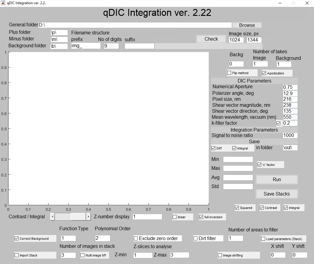
The user should specify the location of datafiles on the hard disk (general folder). Within that folder, the user should create subfolders for raw DIC images taken for positive and negative ellipticity of the incident beam. The absolute value of the incident ellipticity for positive and negative phase should be equal. The user calls the plus ("p") and minus ("m") folder according to the actual file location. The filename is constructed using the current settings of the Hamamatsu camera software. The variable part between prefix and suffix has a fixed number of digits (9 in this case), so the files are img_000000000.tif, img_000000001.tif, etc. User can browse for data folder using "Browse" button, and can check the filename using "Check" button. Note that the prefix, the number of digits and the suffix are all modifiable so that the user may use their own image naming convention (this must contain digits however).
Usually, several takes of each area of the sample are made. The number of takes (1 by default for DIC images) should be specified. The user should measure the average dark counts (plus leakage) value throughout the image and input it in "Backg" field.
Alternatively the user may take background images in order to subtract the dark counts from the DIC images. An error message will appear if no background images are found; the program will still run and use the average dark counts instead. It is not advisable to use both methods of background subtraction at once, which is why the "backg" field is set to 0 by default. If no background images are used, set the "Background" field to 1 (default).
The user can place single multi-image *.tiff files in the \p\ and \m\ folders, and tick the "Multi image tiff" checkbox and input the filename in the manner described above (Files and folders for single z-planes).
The user may also create a stack of integrated images through placing multiple *.tiff images in the \p\ and \m\ folders and unticking the "Multi image tiff" checkbox before hitting "Run". The variable part between the prefix and the suffix changes in a manner described in the section above when the software reads in file names, however the number of images which are read in is limited by the "Number of images in stack" field rather than the "Number of takes" field.
The signal-to-noise ratio influences the amount of integration artefacts, and it changes the magnitude of long-rage features in the image. The user should look at the resulting integrated images and see if the degree of noise is tolerable. The value of 300 was found to be a good trade-off for the Galileo microscope.
Image apodization may be used to remove edge artefacts from the edges of images after integration (through smoothing), and should be used as standard. The "Apodization" tickbox is used to activate this feature.
This feature corrects slowly varying background changes (often seen in the direction of the shear vector), and is activated by a tick box named "Correct Background". For polynomial background subtraction (used as standard) the "Function Type" field should be set to 1 (default value), inputting "2" in this field give exponential polynomial fitting, not used as standard. The Polynomial Order field should be set two 2 (default), although this is also adjustable.
The "Exclude zero order" tickbox can be used to remove the zero order term in the polynomial background correction (not used by default).
The dirt filter functionality is used in order to filter out unwanted objects within images that cause large artefacts in the outputted integrated images (phi). A smoothed array of values within the delta image replaces the area filtered out by the user in order to achieve this. To use this feature tick the "Dirt filter" check box, and specify the number of areas that you wish to filter in the field labelled "Number of areas to filter".
The program saves all resulting files in the subfolder with name given by "in folder" field within the "General folder". Multiple runs of the program will re-write the previous version of the files, so it is recommended to copy them elsewhere or to rename "in folder" location.
User can choose to save differential phase delta and/or integrated phase phi. For each phase, three files are saved: a normalized tiff image, where the minimum is 0 and maximum is 1 (please note the actual min and max values in the corresponding fields of the figure), a *.dat file (ascii), and A *.mat file (binary Matlab format). The dat and mat files contain absolute values of the phase in radians.
If the "Import stack" tick box is unchecked, the contrast and integrated images are saved automatically (as in previous versions).
Stacks are outputted in 16 bit multipage tiff format after analysing stacks and hitting the "Save button" (Stacks will not be saved otherwise!)- these image files are smaller than the 32 bit *.dat files that were outputted in previous versions. The scaling can be seen in the image information that is part of the *.tiff file. To save Contrast, Integral and Squared (Square of integrated images) stacks, tick the check boxes of the same names located under the "Save Stacks" button before hitting "Save Stacks".
These outputted images can then be scaled according to the max values and min values found in the *.tiff file: these are accessible through hitting Ctrl+I in ImageJ.
The parameters used in for each z-plane are saved in a *.mat and *.txt file upon hitting the "Save Stacks" button.
A stack may be analysed by using integration parameters used in a previous analysis session by ticking the "Load parameters (Stack) " checkbox, and hitting "Run".
NOTE: to use parameters saved from previous session on a stack that has not yet been analysed, place a copy of the "Stack_parameters.mat" in a folder named "out" (if the default value for "in folder" is unchanged) - place this folder in the same directory as the "p", "m" and "b" files.
This feature shift the the "p" and "m" images relative to one another in pixel steps to counter the misalignment of objects between images caused by focal drift - this is done by varying the "X shift" and "Y shift" parameters and ticking the "Image shifting" checkbox.
This field is used in order to view analysed data from the current analysis session e.g. to view the integrated image created for the third set of images in a stack input 3 into this field. The values used to integrate this image are also displayed upon varying the value in this field. The "Contrast/Integral" slider may be used to view the contrast and integral images for each z-plane.
The user can specify which z-planes within the stack are to be analysed through using the "Z-min" and "Z-max" fields. Through this function, the user can integrate each (or multiple images) with a particular set of integration parameters.
This feature is an alternative to the apodization routine, contrast images are extended by stitching flipped versions of the input images before Fourier Transforming. This is done in order to minimise aliasing effects by removing discontinuities between the edges of the Fourier Transformed image in both dimesions - this method is suitable for simple objects such as waveguides, but unsuitable for lipid bilayer samples (apodization is the superior option in this case)
This option allows the user to use a linearised version of the equation for extracting differential phase from the composite DIC image as opposed to the fully invertible equation (full inversion is recommended by default).
Spatial frequencies that are above the Nyquist limit of the optical setup can be filtered out using the k-filter - a sinusoidal apodization function is used to smoothly reduce the Fourier amplitudes for spatial frequencies above the k-max value to zero (k-max is the Nyquist limit of the optical system). The k-filter factor defines the range of spatial frequencies over which the apodization function is used. The size of this range is determined through multiplying the k-filter factor with k-max. NOTE: k-max is the central value of the user defined range over which the apodization function is used, so values above and below k-max are apodized and some spatial frequencies above k-max will have a non-zero amplitude. There is a checkbox to enable this feature and it is used by default.
This is a checkbox which is used to make the mean values of the background subtracted positive and negative polarisation DIC images equal through multiplying both images by a factor. This checkbox is checked as default and its use is recommended especially if there is a considerable difference between the mean values of both positive and negative polarisation DIC images.